by Marc-Olivier Jodoin on Unsplash

With the ever-increasing popularity of Amazon’s data warehousing service Redshift, there is a need to understand how this popular and powerful service should be optimised in order to achieve the results expected by its users.

A common misconception with Amazon Redshift is that due to the sheer compute capacity and memory provided by AWS, it is able to churn through millions if not billions of records with ease. This may be true but only if the data has been optimally distributed (read stored), sorted and compressed. In this post we will describe the best practices for storing and sorting data for use in Data Vault, one of the most popular data warehouse modeling practices.

As a side note, Amazon Redshift architecture and any of its underpinnings will not be described in this post. For more information please see Amazon Redshift System Overview.

Firstly before diving into examples, let’s give a brief introduction into the tools provided to us by Amazon Redshift to speed up query performance and enable us to achieve the speeds expected of the service.

Distribution

Distribution of data within Amazon Redshift defines how and where the data will be physically stored in the service. Amazon Redshift provides three distribution styles, Even, Key and, ALL.

Even Distribution The leader node distributes the rows across the slices in a round-robin fashion, regardless of the values in any particular column.

Key Distribution The rows are distributed according to the values in one column. The leader node will attempt to place matching values on the same node slice. If you distribute a pair of tables on the joining keys, the leader node collocates the rows on the slices according to the values in the joining columns so that matching values from the common columns are physically stored together.

ALL Distribution A copy of the entire table is distributed to every node. Where EVEN distribution or KEY distribution place only a portion of a table’s rows on each node, ALL distribution ensures that every row is collocated for every join that the table participates in.

via Distribution Styles

An important note to know here is, when joining two tables with different key distribution styles (except ALL), Amazon Redshift will automatically redistribute all necessary tables by the join key used in the query. In the worst case, both tables will be redistributed, in the best case only the smallest of the two will.

Sorting

Sorting the data tells Amazon Redshift in what order to physically store the data within the service. This information is then fed back to Amazon Redshift’s query planner that utilises this for improved query performance.

Compound Sort Key A compound key is made up of all of the columns listed in the sort key definition, in the order they are listed. The performance benefits of compound sorting decrease when queries depend only on secondary sort columns, without referencing the primary columns. COMPOUND is the default sort type.

Interleaved Sort Key An interleaved sort gives equal weight to each column, or subset of columns, in the sort key. If multiple queries use different columns for filters, then you can often improve performance for those queries by using an interleaved sort style.

via Choosing Sort Keys

Now that we’ve covered the basic theories behind distribution and sorting on Amazon Redshift, let’s dive into a real-world example of how these two concepts should be used to achieve the expected performance for Data Vault.

Hubs & Satellites

Let’s take a basic Data Vault model and break down the performance changes we need to employ.

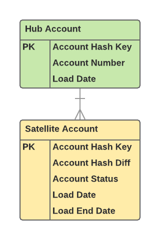
In this example, we have a single Account Hub and its Satellite. The two tables share a common join key, Account Hash Key. This key makes it a perfect choice for Key Distribution as we want the data to be physically co-located whenever joining the two tables together.

When selecting the appropriate sort key, we need to understand the query patterns for the above tables. Query patterns help us define the columns most frequently used by the end user to filter, group and, sort their data. However, since Data Vault is primarily used to populate a Dimensional Model, we generally won’t be sorting on any business related columns. Instead, we’ll use an Interleaved Sort on both the Load Date for the Hub and the Load Date and Load End Date for the Satellite. The reason behind selecting these columns is due to the fact that when selecting data from the Hub and/or Satellite to populate the Dimensional Model we do so in a delta fashion. To save processing time we only select the records that were inserted into the Hub and Satellite since the last time the tables were accessed to populate the Dimensional Model.

Hubs, Links & Satellites

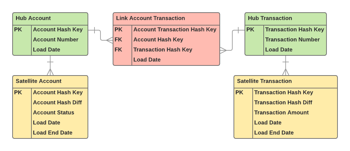
Now let’s take a look at a more complex example by throwing a Link in the mix. The new Transaction Hub and Satellite will be distributed and sorted in the exact same manner the Account Hub and Satellite were (based on their respective Hash Keys). But the Link now has two different joins. It joins to the Account Hub and the Transaction Hub. Here it gets a little tricky. We want the join between the two Hubs and the Link to be as performant as possible, but we must sacrifice one of the joins performance in order to benefit from the other.

The simple rule is, the biggest table always wins

If we assume the Account Hub contains 100,000 records and the Transaction Hub contains 1,000,000 records, we distribute the Account Transaction Link on the Transaction Hash Key. The reason for this is we would rather have Amazon Redshift redistribute the Account Hub to match the distribution of the Account Transaction Link than have the Transaction Hub do so due to the larger number of records.

Redistribution of data is a very costly exercise within Amazon Redshift and lowering the cost of that distribution will inevitably lead to better performance. It is worth noting that as your Data Vault grows, tables might that were expected to contain less data may eventually overtake those that were expected to have more data. In scenarios such as these ones distribution styles or keys should be altered to ensure peak performance is maintained.

Rules to Follow

1. For tables under 10,000 (maybe even up to 100,000) records (generally tables containing reference data), use ALL Distribution. These tables can have multiple join keys to multiple tables of which will generally not be distributed on the same keys.

2. For tables over 10,000 records (generally not reference data), use Key Distribution.

3. Always distribute on the most frequently used high cardinality join key. For Hubs and Satellites, this is the Hash Key. For Links, this is the the Hash Key of the largest Hub the Link joins with.

4. Frequently check table sizes and distribution styles/keys to ensure optimal join performance is maintained as table growth may have exceeded initial estimates done during the profiling stage.

5. As a general rule, Interleaved Sort Keys are more preferable as they provide greater flexibility compared to Compound Sort Keys.

6. Sort keys should be selected based on the most commonly used columns when filtering, ordering or grouping the data. For Hubs and Links this is the Load Date. For Satellites this is the Load Date and Load End Date. Other columns may also be added such as Account Status as it may be useful to only select active accounts. This therefore makes sense for the column to be added to the sort key.

For more information see Amazon Redshift Engineering’s Advanced Table Design Playbook: Distribution Styles and Distribution Keys for a great in-depth write up on this topic and more.